Creating NIF files from SDTM data • nif

INTRODUCTION

This is a basic tutorial on using the nif package to create NONMEM Input File (NIF) data sets from Study Data Tabulation Model- (SDTM) formatted data.

Background

Following regulatory standards, clinical study data are commonly provided in SDTM format, an observation-based data tabulation format in which logically related observations are organized into topical collections (domains). SDTM is defined and maintained by the Clinical Data Interchange Standards Consortium (CDISC).

To support typical pharmacometric analyses, data from different SDTM domains need to be aggregated into a single analysis data set. For example, demographic and pharmacokinetic concentration data from the DM and PC domains are both required to evaluate exposure by age. More complex analyses like population-level PK and PK/PD analyses may include further data, e.g., clinical laboratory, vital sign, or biomarker data.

NONMEM and other modeling software packages expect the input data provided in (long) tabular arrangement with strict requirements to the formatting and nomenclature of the variables (see, e.g., Bauer, CPT Pharmacometrics Syst. Pharmacol. (2019) for an introduction). The input data file for these analyses is sometimes casually referred to as a ‘NONMEM input file’ or ‘NIF file’, hence the name of this package.

Contingent on the downstream analyses, some of the variables in the analysis data set can be easily and automatically derived from the SDTM source data, e.g., ‘DOSE’ (the administered dose) or ‘DV’ (the dependent variable for observations), or demographic covariates like ‘AGE’, ‘SEX’ or ‘RACE’. Other fields of the input data set may require study-specific considerations, for example the calculation of baseline renal or hepatic function categories, definition of specific treatment conditions by study arm, or the encoding of adverse events or concomitant medications, as categorical covariates.

While the latter variables often need manual and study-specific data programming, the core NIF data set can in most cases be generated in a quite standardized way. Both approaches are substantially made easier by the functions that the nif package provides. Often, analysis data sets can be created with only a handful of lines of code.

It should be noted that even for basic NIF files, missing data points or data inconsistencies are challenges that need to be resolved by data imputation to get to analysis-ready data sets. This is frequently encountered when analyzing preliminary data from ongoing clinical studies that have not been fully cleaned yet. The nif package provides a number of standardized imputation rules to resolve these issues. More on this point later as well in a separate vignette (vignette("nif-imputations")).

This package is intended to facilitate the creation of analysis data sets (‘NIF data sets’) from SDTM-formatted clinical data. It also includes a set of functions and tools to support initial exploration of SDTM and NIF data sets.

Outline

The first part of this tutorial describes how to import SDTM data into a sdtm object, and how to explore clinical data on the SDTM level.

The second part walks through the generation of a sample nif data set from SDTM data to illustrate the general workflow for building analysis data sets.

Finally, the third part showcases some functions to quickly explore analysis data sets.

This tutorial contains live code that depends on the following R packages:

library(tidyr)
library(dplyr)
library(stringr)
library(nif)

SDTM DATA

Importing SDTM data

In most cases, the source SDTM data are provided as one file per domain, e.g., in SAS binary data base storage format (.sas7bdat) or SAS Transport File (.xpt) format.

With path/to/sdtm/data the location to the source folder, SDTM data can be loaded using read_sdtm():

read_sdtm("path/to/sdtm/data")

Windows users may want to provide the file path as raw string, i.e., in the form of

read_sdtm(r"(path\to\sdtm\data)")

to ensure that the backslashes in the file path are correctly captured. Note the inner parentheses around the file path!

If no domains are explicitly specified, the function attempts to load ‘DM’, ‘VS’, ‘EX’ and ‘PC’ as a generic set of SDTM domains suitable to create a basic pharmacokinetic analysis data set.

The return value of this function is a sdtm object.

SDTM objects

sdtm objects are essentially aggregates (lists) of the SDTM domains from a particular clinical study, plus some metadata. The easiest way of creating sdtm objects is by importing the SDTM data using read_sdtm() as shown above.

The nif package includes sample SDTM data sets for demonstration purposes. These data do not come from actual clinical studies but are fully synthetic data sets from a fictional single ascending dose (SAD) study (examplinib_sad), a fictional food effect (FE) study (examplinib_fe), and a fictional single-arm proof-of-concept (POC) study with multiple-dose administrations (examplinib_poc).

The original SDTM data can be retrieved from sdtm objects by accessing the individual SDTM domains like demonstrated below for the DM domain of the examplinib_fe data object:

domain(examplinib_sad, "dm") %>% 
  head(3)
#>   SITEID  SUBJID                              ACTARM ACTARMCD          RFICDTC
#> 1    101 1010001 Treatment cohort 1, 5 mg examplinib       C1 2000-12-21T10:18
#> 2    101 1010002 Treatment cohort 1, 5 mg examplinib       C1 2000-12-21T10:30
#> 3    101 1010003 Treatment cohort 1, 5 mg examplinib       C1 2000-12-21T09:22
#>            RFSTDTC         RFXSTDTC    STUDYID           USUBJID SEX AGE  AGEU
#> 1 2000-12-31T10:18 2000-12-31T10:18 2023000001 20230000011010001   M  43 YEARS
#> 2 2000-12-29T10:30 2000-12-29T10:30 2023000001 20230000011010002   M  49 YEARS
#> 3 2000-12-29T09:22 2000-12-29T09:22 2023000001 20230000011010003   M  46 YEARS
#>   COUNTRY DOMAIN                                 ARM ARMCD
#> 1     DEU     DM Treatment cohort 1, 5 mg examplinib    C1
#> 2     DEU     DM Treatment cohort 1, 5 mg examplinib    C1
#> 3     DEU     DM Treatment cohort 1, 5 mg examplinib    C1
#>                        RACE ETHNIC          RFENDTC
#> 1                     WHITE        2000-12-31T10:18
#> 2                     WHITE        2000-12-29T10:30
#> 3 BLACK OR AFRICAN AMERICAN        2000-12-29T09:22

Printing an sdtm object shows relevant summary information:

examplinib_fe
#> -------- SDTM data set summary -------- 
#> Study 2023000400 
#> 
#> Data disposition
#>   DOMAIN   SUBJECTS   OBSERVATIONS   
#>   dm       28         28             
#>   vs       28         56             
#>   ex       20         40             
#>   pc       20         1360           
#>   lb       28         28             
#>   pp       20         360            
#> 
#> Arms (DM):
#>   ACTARMCD   ACTARM           
#>   SCRNFAIL   Screen Failure   
#>   BA         Fed - Fasted     
#>   AB         Fasted - Fed     
#> 
#> Treatments (EX):
#>   EXAMPLINIB
#> 
#> PK sample specimens (PC):
#>   PLASMA
#> 
#> PK analytes (PC):
#>   PCTEST       PCTESTCD     
#>   RS2023       RS2023       
#>   RS2023487A   RS2023487A

Note the ‘Treatment-to-analyte mappings’ table in the output, we may get back to this in the context of automatically creating NIF data sets.

High-level subject-level disposition data can be extracted using subject_info():

examplinib_fe %>%
  subject_info("20230004001050001")
#>          [,1]                     
#> SITEID   105                      
#> SUBJID   1050001                  
#> ACTARM   Fasted - Fed             
#> ACTARMCD AB                       
#> RFICDTC  2000-12-26T10:05         
#> RFSTDTC  2001-01-05T10:05         
#> RFXSTDTC 2001-01-05T10:05         
#> STUDYID  2023000400               
#> USUBJID  20230004001050001        
#> SEX      M                        
#> AGE      34                       
#> AGEU     YEARS                    
#> COUNTRY  DEU                      
#> DOMAIN   DM                       
#> ARM      Fasted - Fed             
#> ARMCD    AB                       
#> RACE     BLACK OR AFRICAN AMERICAN
#> ETHNIC                            
#> RFENDTC  2001-01-18T10:05

For a broad-strokes overview on the overall data disposition, it may be informative to look at a timeline view of individual domains, e.g. for DM:

plot(examplinib_fe, "dm")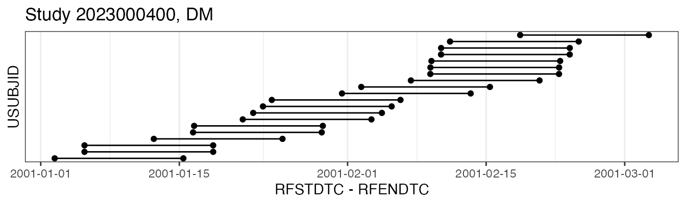

SDTM suggestions

SDTM data may be incomplete, e.g., when emerging data that have not yet been fully cleaned are analyzed. In addition, some study-specific data may be encoded in a non-standardized way, e.g., information on study parts, cohorts, treatment conditions, etc..

Such data fields may need study-specific considerations and manual imputations during the creating of the analysis data set. To help deciding which study-specific factors need to be addressed, the nif package includes functions to explore the structure of SDTM data.

As a starting point, suggest() can provide useful suggestions for the creation of analysis data sets:

suggest(examplinib_fe)
#> 1. There are 1 different treatments in 'EX' (see below).
#>       EXTRT        
#>       ----------
#>       EXAMPLINIB
#>    Consider adding them to the nif object using `add_administration()`, see the
#>    code snippet below (replace 'sdtm' with the name of your sdtm object):
#>    ---
#>      %>%
#>        add_administration(sdtm, 'EXAMPLINIB')
#>    ---
#> 2. There are 2 different pharmacokinetic analytes in 'PC':
#>       PCTEST       PCTESTCD     
#>       ----------   ----------
#>       RS2023       RS2023       
#>       RS2023487A   RS2023487A
#>    Consider adding them to the nif object using `add_observation()`. Replace
#>    'sdtm' with the name of your sdtm object and 'y' with the respective
#>    treatment code (EXAMPLINIB):
#>    ---
#>      %>%
#>        add_observation(sdtm, 'pc', 'RS2023', parent = 'y') %>%
#>        add_observation(sdtm, 'pc', 'RS2023487A', parent = 'y')
#>    ---
#> 3. There are 3 arms defined in DM (see below). Consider defining a PART or ARM
#>    variable in the nif dataset, filtering for a particular arm, or defining a
#>    covariate based on ACTARMCD.
#>       ACTARM           ACTARMCD   
#>       --------------   --------
#>       Screen Failure   SCRNFAIL   
#>       Fed - Fasted     BA         
#>       Fasted - Fed     AB

Suggestions 1 and 2 in the above output include code snippets for the creation of a nif object from this sdtm data set. We will use this code straight out-of-the box in section [Creating NIF data sets].

Suggestion 3 notes that the DM domain defines different treatment arms that should probably be included as covariates in the analysis data set because they specify the sequence of fasted and fed administrations in this study. We will deal with this in Study-specific covariates.

NIF DATA SETS

The following sections continue using the examplinib_fe example to demonstrate how a nif object is created from the sdtm data object.

Basic NIF file

Based on the analysis needs, nif objects are assembled in a stepwise manner, starting from an empty nif object, adding treatment administrations, observations, and covariate fields. The result is a data table with individual rows for administrations and observations that follows the naming conventions summarized in Bauer, CPT Pharmacometrics Syst. Pharmacol. (2019).

The basic nif object automatically includes standard demographic parameters as subject-level covariates: SEX, AGE and RACE, and baseline WEIGHT and HEIGHT are taken from the DM and VS domains, respectively, and merged into the data set as columns of those names:

sdtm <- examplinib_fe

nif <- new_nif() %>% 
  add_administration(sdtm, "EXAMPLINIB", analyte = "RS2023") %>% 
  add_observation(sdtm, "pc", "RS2023")

Note that in this SDTM data, the name of the treatment, i.e., the value of the ‘EXTRT’ field is ‘EXAMPLINIB’ while the pharmacokinetic analyte name (PCTESTCD) is ‘RS2023’. To harmonize both, the ‘analyte’ parameter in add_administration() was set to ‘RS2023’, too.

These are the first rows of the resulting data table:

head(nif, 5)
#>   REF ID    STUDYID           USUBJID AGE SEX  RACE HEIGHT WEIGHT      BMI
#> 1   1  1 2023000400 20230004001010002  53   1 WHITE  180.4   73.1 22.46179
#> 2   2  1 2023000400 20230004001010002  53   1 WHITE  180.4   73.1 22.46179
#> 3   3  1 2023000400 20230004001010002  53   1 WHITE  180.4   73.1 22.46179
#> 4   4  1 2023000400 20230004001010002  53   1 WHITE  180.4   73.1 22.46179
#> 5   5  1 2023000400 20230004001010002  53   1 WHITE  180.4   73.1 22.46179
#>                   DTC TIME NTIME TAFD TAD EVID AMT ANALYTE CMT PARENT TRTDY
#> 1 2001-01-05 10:05:00  0.0     0  0.0 0.0    1 500  RS2023   1 RS2023     1
#> 2 2001-01-05 10:05:00  0.0     0  0.0 0.0    0   0  RS2023   2 RS2023     1
#> 3 2001-01-05 10:35:00  0.5    NA  0.5 0.5    0   0  RS2023   2 RS2023     1
#> 4 2001-01-05 11:05:00  1.0    NA  1.0 1.0    0   0  RS2023   2 RS2023     1
#> 5 2001-01-05 11:35:00  1.5    NA  1.5 1.5    0   0  RS2023   2 RS2023     1
#>   METABOLITE DOSE MDV ACTARMCD IMPUTATION       DV
#> 1      FALSE  500   1       AB                  NA
#> 2      FALSE  500   0       AB               0.000
#> 3      FALSE  500   0       AB            4697.327
#> 4      FALSE  500   0       AB            6325.101
#> 5      FALSE  500   0       AB            6294.187

Multiple analytes

To demonstrate how to add multiple analytes to a nif object, we will temporarily switch to another built-in sample data set, examplinib_sad. This sdtm object includes pharmacokinetic concentration data for the M1 metabolite of ‘EXAMPLINIB’ under the PCTESTCD of ‘RS2023487A’. Note how in the below code, the respective observations are attached to the data set, setting the name to ‘M1’, and how the relation to the parent compound is established using the ‘parent’ parameter:

sdtm1 <- examplinib_sad

nif1 <- new_nif() %>% 
  add_administration(sdtm, "EXAMPLINIB", analyte = "RS2023") %>% 
  add_observation(sdtm, "pc", "RS2023") %>% 
  add_observation(sdtm, "pc", "RS2023487A", analyte = "M1", parent = "RS2023")

In analogy to PK observations, observations from any SDTM domain, e.g., LB, VS, MB, TR, etc., can be added in very much the same way. Please see the documentation to add_observation() for details. This is a powerful feature that allows effortless construction of analysis data sets for population PK/PD modeling.

Study-specific covariates

In this study, participants received the test drug, EXAMPLINIB, fasted or fed in a randomized sequence (see ACTARM and ACTARMCD in the output of suggest()), where the ‘EPOCH’ field in ‘EX’ provides information on the current treatment period. It should be noted that the way such information is encoded in the SDTM data varies considerably. This is therefore only an example - the specifics of how covariate information can extracted from a SDTM data set will differ. However, nif objects are essentially data frame objects and can thus be easily manipulated, e.g., using functions from the dplyr package.

The following code shows how in this specific case, covariates relating to the current treatment period (‘PERIOD’) and current treatment (‘TREATMENT’) are sequentially derived and eventually used to create the ‘FASTED’ covariate.

Note that the ‘EPOCH’ field is not carried over from ‘EX’ to the nif object by default, but needs to be added using the ‘keep’ parameter to add_observation():

nif <- new_nif() %>% 
  add_administration(sdtm, "EXAMPLINIB", analyte = "RS2023") %>% 
  add_observation(sdtm, "pc", "RS2023", keep = "EPOCH") %>% 
  mutate(PERIOD = str_sub(EPOCH, -1, -1)) %>% 
  mutate(TREATMENT = str_sub(ACTARMCD, PERIOD, PERIOD)) %>% 
  mutate(FASTED = case_when(TREATMENT == "A" ~ 1, .default = 0))

These are again the first 5 lines:

head(nif, 5)
#>   REF ID    STUDYID           USUBJID AGE SEX  RACE HEIGHT WEIGHT      BMI
#> 1   1  1 2023000400 20230004001010002  53   1 WHITE  180.4   73.1 22.46179
#> 2   2  1 2023000400 20230004001010002  53   1 WHITE  180.4   73.1 22.46179
#> 3   3  1 2023000400 20230004001010002  53   1 WHITE  180.4   73.1 22.46179
#> 4   4  1 2023000400 20230004001010002  53   1 WHITE  180.4   73.1 22.46179
#> 5   5  1 2023000400 20230004001010002  53   1 WHITE  180.4   73.1 22.46179
#>                   DTC TIME NTIME TAFD TAD EVID AMT ANALYTE CMT PARENT TRTDY
#> 1 2001-01-05 10:05:00  0.0     0  0.0 0.0    1 500  RS2023   1 RS2023     1
#> 2 2001-01-05 10:05:00  0.0     0  0.0 0.0    0   0  RS2023   2 RS2023     1
#> 3 2001-01-05 10:35:00  0.5    NA  0.5 0.5    0   0  RS2023   2 RS2023     1
#> 4 2001-01-05 11:05:00  1.0    NA  1.0 1.0    0   0  RS2023   2 RS2023     1
#> 5 2001-01-05 11:35:00  1.5    NA  1.5 1.5    0   0  RS2023   2 RS2023     1
#>   METABOLITE DOSE MDV ACTARMCD IMPUTATION       DV                  EPOCH
#> 1      FALSE  500   1       AB                  NA OPEN LABEL TREATMENT 1
#> 2      FALSE  500   0       AB               0.000 OPEN LABEL TREATMENT 1
#> 3      FALSE  500   0       AB            4697.327 OPEN LABEL TREATMENT 1
#> 4      FALSE  500   0       AB            6325.101 OPEN LABEL TREATMENT 1
#> 5      FALSE  500   0       AB            6294.187 OPEN LABEL TREATMENT 1
#>   PERIOD TREATMENT FASTED
#> 1      1         A      1
#> 2      1         A      1
#> 3      1         A      1
#> 4      1         A      1
#> 5      1         A      1

DATA EXPLORATION

Data disposition

It is generally an excellent idea to explore data sets before proceeding into more complex analyses. The nif package provides a host of functions to this end. The following section provides some basic examples.

The summary() function generates a general overview on the data disposition in a nif data set:

summary(nif)
#> ----- NONMEM input file (NIF) object summary -----
#> Data from 20 subjects across one study:
#>   STUDYID      N    
#>   2023000400   20   
#> 
#> Sex distribution:
#>   SEX      N    percent   
#>   male     13   65        
#>   female   7    35        
#> 
#> Treatments:
#>   RS2023
#> 
#> Analytes:
#>   RS2023
#> 
#> Subjects per dose level:
#>   RS2023   N    
#>   500      20   
#> 
#> 680 observations:
#>   CMT   ANALYTE   N     
#>   2     RS2023    680   
#> 
#> Subjects with dose reductions
#>   RS2023   
#>   2        
#> 
#> Treatment duration overview:
#>   PARENT   min   max   mean   median   
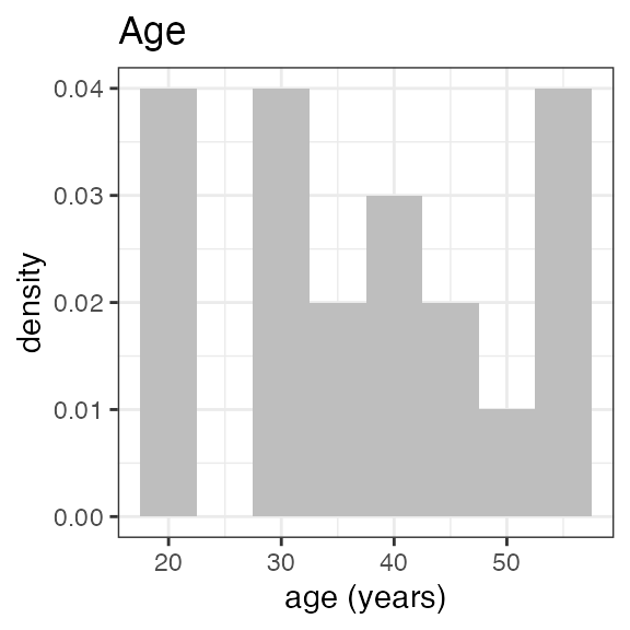
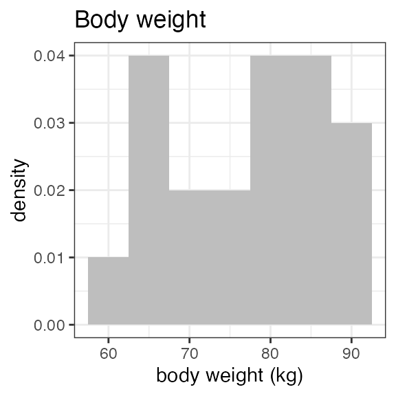
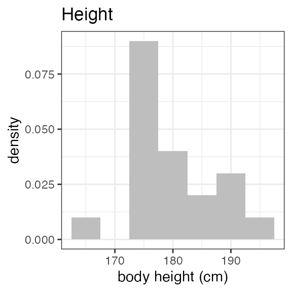
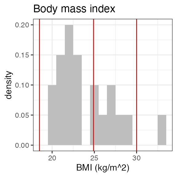
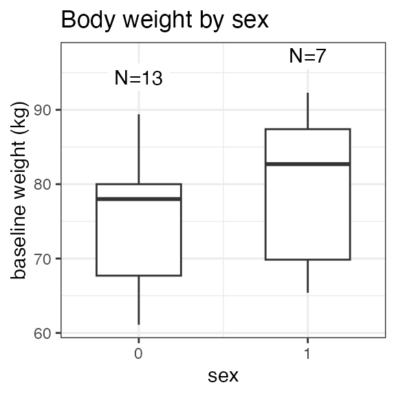
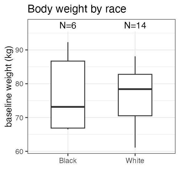
#>   RS2023   2     2     2      2

Plotting the summary yields histograms of the baseline demographic covariates and raw plots of the analytes over time. In the following code, ignore the ìnvisible(capture.output()) construct around the plot() function. Its sole purpose is to omit some non-graphical output:

invisible(capture.output(
  nif %>% 
    summary() %>% 
    plot()
))

#> Warning in transformation$transform(x): NaNs produced
#> Warning in ggplot2::scale_y_log10(): log-10 transformation
#> introduced infinite values.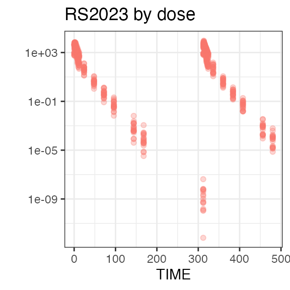

Plasma concentration data

nif objects can be easily plotted as time series charts using the generic plot() function. While the output is a standard ggplot2 object that can be further extended using ggplot2 functionality, the plot() function itself includes extensive parameters to achieve the desired data visualization.

In its simplest form, plot() includes all analytes, and uses ‘time after first dose’ (‘TAFD’) as the time metric:

plot(nif)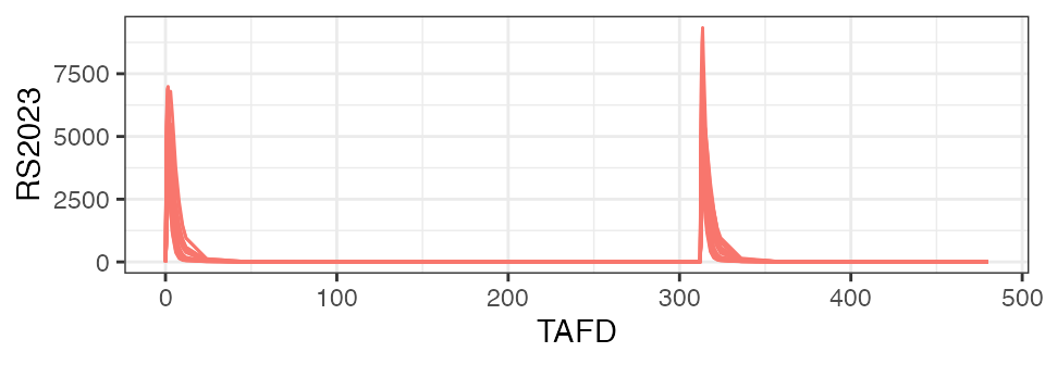

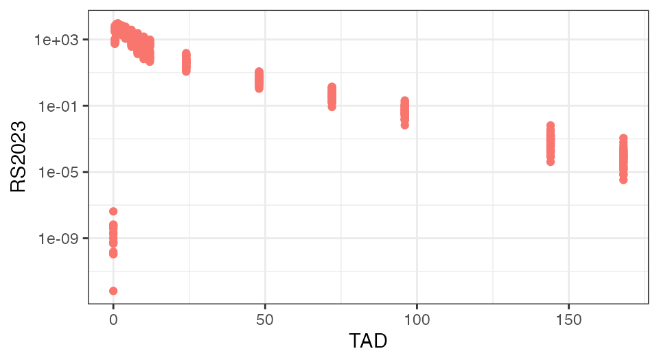
To check the integrity of the data set, if often helps to plot the analyte concentrations over time-after-dose (TAD):

nif %>% 
  plot(time="TAD", points=TRUE, lines=FALSE, log=TRUE)

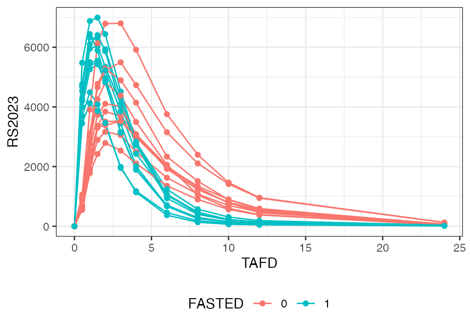
To demonstrate the food effect on Cmax and Tmax on the individual level, the below figure focuses on the first 24 hours on the linear scale and introduces coloring based on the ‘FASTED’ covariate field:

nif %>% 
  plot(color="FASTED", max_time=24, points=TRUE)

The following compares the mean plasma concentration profiles:

nif %>% 
  plot(color="FASTED", max_time=24, mean=TRUE, points=TRUE)
#> `geom_line()`: Each group consists of only one observation.
#> ℹ Do you need to adjust the group aesthetic?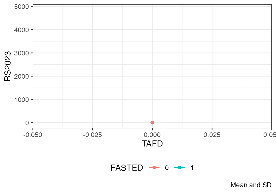

Refer to the documentation (?plot.nif()) for further options.

NIF viewer

nif_viewer() is a powerful exploratory tool that lets you interactively explore all analyte profiles on an individual level. As the static nature of a vignette does not allow to fully appreciate its potential, you are encouraged to test nif_viewer() within your RStudio.

nif_viewer(nif)