Importing NIF data sets • nif

INTRODUCTION

NIF data can be imported
nif objects by default contain more information than minimally required by the NONMEM specification
ANALYTE, PARENT, DOSE and TAFD fields are automatically generated
other fields may be derived by renaming terms

The code in this vignette depends on the following packages:

library(dplyr)
library(nif)

For this demonstration, we use a minimal nif dataset that contains data from 2 subjects with single administrations into compartment 1, and observations up to 6 hours from compartment 2:

ID,TIME,AMT,RATE,EVID,DV,CMT,MDV
1,0,5,0,1,.,1,1
1,0,0,0,0,0,2,0
1,0.5,0,0,0,0.0024,2,0
1,1,0,0,0,0.0072,2,0
1,1.5,0,0,0,0.0157,2,0
1,2,0,0,0,0.0209,2,0
1,3,0,0,0,0.0148,2,0
1,4,0,0,0,0.0133,2,0
1,6,0,0,0,0.0055,2,0
2,0,5,0,1,.,1,1
2,0,0,0,0,0,2,0
2,0.5,0,0,0,0.0036,2,0
2,1,0,0,0,0.0128,2,0
2,1.5,0,0,0,0.0228,2,0
2,2,0,0,0,0.0272,2,0
2,3,0,0,0,0.0256,2,0
2,4,0,0,0,0.0197,2,0
2,6,0,0,0,0.0117,2,0

The dataset contains the minimally expected columns, ID, TIME, AMT, RATE, EVID, DV, CMT, MDV, and is provided as a csv file (csv_file_name).

IMPORTING NIF DATA

The external data can be imported as a nif object using import_nif():

nif <- import_nif(csv_file_name, format = "csv")
head(nif)
#>   REF ID TIME EVID AMT CMT MDV RATE     DV
#> 1   1  1  0.0    1   5   1   1    0     NA
#> 2   2  1  0.0    0   0   2   0    0 0.0000
#> 3   3  1  0.5    0   0   2   0    0 0.0024
#> 4   4  1  1.0    0   0   2   0    0 0.0072
#> 5   5  1  1.5    0   0   2   0    0 0.0157
#> 6   6  1  2.0    0   0   2   0    0 0.0209

The resulting object behaves as a regular nif object, for example, it can be summarized or plotted or otherwise explored (see vignette("nif-tutorial") for more information):

summary(nif)
#> ----- NONMEM Input Format (NIF) data summary -----
#> Data from 2 subjects across 0 studies:
#>   N   
#>   2    
#> 
#> Sex distribution:
#>   SEX      N   percent   
#>   male     0   0         
#>   female   0   0         
#>   NA       2   100        
#> 
#> Treatments:
#>   CMT1
#> 
#> Analytes:
#>   CMT2
#> 
#> Subjects per dose level:
#>   CMT1   N   
#>   5      2    
#> 
#> 16 observations:
#>   CMT   N    
#>   2     16    
#> 
#> Subjects with dose reductions
#>   CMT1   
#>   0       
#> 
#> Treatment duration overview:
#>   PARENT   min   max   mean   median   
#>   CMT1     1     1     1      1         
#> 
#> Hash: c03cb2ca160fb8dfbb480ce8dc7d965f
plot(nif, log = T, points = T)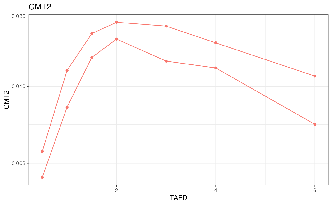

Transformations

In some cases, the data to be imported include columns that should be renamed or transformed to match the desired naming conventions, or to otherwise support downstream analyses.

For this demonstration, let’s assume that the ‘TIME’ field in the csv file is also the nominal time, and we want to include it in the nif object as ‘NTIME’. in addition, the values in DV should be transformed from ng/ml to micromolar concentrations (assuming a MW of 400 g/mol). import_nif() allows these transformations to be executed during the data import. Transformation terms need to be provided in the form of new_field ~ transformation_term:

nif <- import_nif(
  csv_file_name,
  format = "csv",
  NTIME ~ TIME,
  DV ~ DV/400
)

head(nif)
#>   REF ID TIME NTIME EVID AMT CMT MDV RATE        DV
#> 1   1  1  0.0   0.0    1   5   1   1    0        NA
#> 2   2  1  0.0   0.0    0   0   2   0    0 0.000e+00
#> 3   3  1  0.5   0.5    0   0   2   0    0 6.000e-06
#> 4   4  1  1.0   1.0    0   0   2   0    0 1.800e-05
#> 5   5  1  1.5   1.5    0   0   2   0    0 3.925e-05
#> 6   6  1  2.0   2.0    0   0   2   0    0 5.225e-05